Applying machine learning to guide ensemble curation

An ensemble of models can be though of as a set of feasible hypotheses about how a system behaves. From a machine learning perspective, these hypotheses can alternatively be viewed as samples (or observations), each of which has a distinct set of features (i.e. the model components that vary across an ensemble) and can further generate new features by performing simulations. An example of the analyses enabled by this view of ensembles can be found in Medlock & Papin, where ensemble structure and ensemble simulations are used to identify reactions that are high-priority targets for curation.

In this example, we demonstrate how ensembles of genome-scale metabolic models and machine learning can be combined to identify reactions that might strongly influence a single prediction (flux through biomass). We will use an ensemble for Staphylococcus aureus that contains 1000 members. The ensemble was generated through iterative gapfilling to enable growth on single C/N media conditions using a draft reconstruction from ModelSEED.

import medusa
from medusa.test import create_test_ensemble

ensemble = create_test_ensemble("Staphylococcus aureus")

Using the ensemble, we’ll perform flux balance analysis and return flux through the biomass reaction (which has an ID of "bio1"). The ensemble already has the media conditions set as “complete”, meaning the boundary reactions for all transportable metabolites are open (e.g. the lower bound of all exchange reactions is -1000).

from medusa.flux_analysis import flux_balance
biomass_fluxes = flux_balance.optimize_ensemble(ensemble, return_flux="bio1", num_processes = 4)

The optimize_ensemble function returns a pandas DataFrame, where each column is a reaction and each row is an ensemble member. For illustration, here are the values for the first 10 members of the ensemble:

biomass_fluxes.head(10)

	bio1
Staphylococcus aureus_gapfilled_518	118.238182
Staphylococcus aureus_gapfilled_860	122.523063
Staphylococcus aureus_gapfilled_900	104.905551
Staphylococcus aureus_gapfilled_434	148.353976
Staphylococcus aureus_gapfilled_343	134.100850
Staphylococcus aureus_gapfilled_706	116.982207
Staphylococcus aureus_gapfilled_175	137.352545
Staphylococcus aureus_gapfilled_85	110.488964
Staphylococcus aureus_gapfilled_345	119.439103
Staphylococcus aureus_gapfilled_161	118.237318

To get a sense for the distribution of biomass flux predictions, we can visualize them with matplotlib:

import matplotlib.pylab as plt
fig, ax = plt.subplots()
plt.hist(biomass_fluxes['bio1'], bins = 15, color = 'black', alpha = 0.4)
ax.set_ylabel('# ensemble members')
ax.set_xlabel('Flux through biomass reaction')
plt.savefig('pre_FBA_curation.svg')
plt.show()

As you can see, there is quite a bit of variation in the maximum flux through biomass! Keep in mind that this is an ensemble of gapfilled reconstructions with no manual curation, and that none of the uptake rates are reallistically constrained, so these predictions are unrealistically high (100 units of flux through biomass is a doubling time of 36 seconds, at least an order of magnitude faster than even the fittest E. coli grown in vitro).

Our goal now is to identify which features in the ensemble are predictive of flux through biomass. If we can identify these reactions, then turn to the literature or perform an experiment to figure out whether they are really catalyzed by the organism, we can greatly reduce the uncertainty in our predictions of biomass flux!

Given that we have a continous output, our problem can be addressed using regression. We will use the binary presence/absence of each reaction in each member of the ensemble as input to a random forest regressor, implemented in scikit-learn. Many supervised regression models will work for this analysis, but random forest is particularly easy to understand and interpret when the input is binary (i.e. reaction presence/absence).

import sklearn
from sklearn.ensemble import RandomForestRegressor

We reformat the data here, getting the feature states for each ensemble member and converting them to True/False, then combine them into a single DataFrame with the biomass flux predictions for matched members.

# Grab the features and states for the ensemble and convert to a dataframe
import pandas as pd
feature_dict = {}
for feature in ensemble.features:
    feature_dict[feature.id] = feature.states
feature_frame = pd.DataFrame.from_dict(feature_dict)
# convert the presence and absence of features to a boolean value
feature_frame = feature_frame.astype(bool)
# extract biomass and add it to the dataframe, keeping track of the feature names
input_cols = feature_frame.columns
biomass_fluxes.index = [member_id for member_id in biomass_fluxes.index]
feature_frame['bio1'] = biomass_fluxes['bio1']

Now we actually construct and fit the random forest regressor, using 100 total trees in the forest. The oob_score_ reported here is the coefficient of determination (R2) calculated using the out-of-bag samples for each tree. As a reminder, R2 varies from 0 to 1.0, where 1.0 is a perfect fit.

# create a regressor to predict biomass flux from reaction presence/absence
regressor = RandomForestRegressor(n_estimators=1000,oob_score=True)
fit_regressor = regressor.fit(X=feature_frame[input_cols],y=feature_frame['bio1'])
fit_regressor.oob_score_

0.8684706250117109

With a reasonably-performing regressor in hand, we can inspect the important features to identify reactions that contribute to uncertainty in biomass flux predictions.

imp_frame = pd.DataFrame(fit_regressor.feature_importances_,
                        index=feature_frame[input_cols].columns).sort_values(
                        by=0,ascending=False)
imp_frame.columns = ['importance']

imp_frame.head(10)

	importance
rxn01640_c_upper_bound	0.129785
rxn01640_c_lower_bound	0.113434
rxn12585_c_lower_bound	0.044854
rxn12585_c_upper_bound	0.042830
rxn15617_c_lower_bound	0.039388
rxn23244_c_lower_bound	0.039336
rxn00602_c_lower_bound	0.037124
rxn15617_c_upper_bound	0.036253
rxn00602_c_upper_bound	0.032443
rxn23244_c_upper_bound	0.028802

With the list of important features in hand, the first thing we should do is turn to the literature to see if someone else has already figured out whether these reactions are present or absent in Staphylococcus aureus. The top reaction, rxn01640, is N-Formimino-L-glutamate iminohydrolase, which is part of the histidine utilization pathway. A quick consultation with a review on the regulation of histidine utilization in bacteria suggests that the enzyme for this reaction, encoded by the hutF gene, is widespread and conserved amongst bacteria. However, the hutF gene is part of a second, less common pathway that branches off of the primary histidine utilization pathway. If we consult PATRIC with a search for the *hutF* gene, we see that, although the gene is widespread, there is no predicted hutF gene in any sequenced Staphylococcus aureus genome. Although absence of evidence is not evidence of absence, we can be relatively confident that hutF is not encoded in the Staphylococcus aureus genome, given how well-studied this pathogen is.

What happens if we “correct” this issue in the ensemble? Let’s inactivate the lower and upper bound for the reaction in all the members, then perform flux balance analysis again.

for member in ensemble.features.get_by_id('rxn01640_c_lower_bound').states:
    ensemble.features.get_by_id('rxn01640_c_lower_bound').states[member] = 0
    ensemble.features.get_by_id('rxn01640_c_upper_bound').states[member] = 0

biomass_fluxes_post_curation = flux_balance.optimize_ensemble(ensemble, return_flux="bio1", num_processes = 4)

import matplotlib.pylab as plt
import numpy as np
fig, ax = plt.subplots()
# declare specific bins for our histogram
bins=np.histogram(np.hstack((biomass_fluxes['bio1'],biomass_fluxes_post_curation['bio1'])),
                  bins=15)[1]
plt.hist(biomass_fluxes['bio1'],
         bins,
         label = 'Original',
         alpha = 0.3,
         color='black')
plt.hist(biomass_fluxes_post_curation['bio1'],
         bins,
         label = 'Post-curation',
         alpha = 0.4,
         color = 'green')
plt.axvline(x=biomass_fluxes['bio1'].mean(), c = 'black', alpha = 0.6)
plt.axvline(x=biomass_fluxes_post_curation['bio1'].mean(), c = 'green')
ax.set_ylabel('# ensemble members')
ax.set_xlabel('Flux through biomass reaction')
plt.legend(loc='upper right')
plt.savefig('post_FBA_curation.svg')
plt.savefig('post_FBA_curation.png')
plt.show()

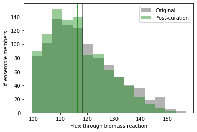
Here, we show the old distribution in gray and the new distribution in green, with vertical lines at the mean in the same color. As you can see, by resolving the identity of the hutF-encoded enzyme, we’ve reduced the mean and range of predicted flux through biomass. The reduction here is modest, but the process can be repeated for the other important features we identified to continue to refine the distribution and improve the reconstruction in a rational way.